Project area/S
- Transient Universe : fast radio bursts (FRBs), pulsars
Project Details
Fast Radio Bursts (FRB) are one of the most intriguing transient phenomena discovered only 15 years ago. Recent localisations and redshift measurements of several FRBs confirmed their extra-galactic origin and extreme energies of the order of 1039 ergs, which are emitted over millisecond intervals. However, full understanding of FRB sources and underlying physical mechanisms powering these extreme events still awaits full explanation. Although FRBs were discovered and initially observed at frequencies around 1.4 GHz, in the last few years several FRBs have been detected down to very low frequencies (even 110-MHz). Multiple detections by Canadian CHIME telescope extending down to 400 MHz, LOFAR detections of repeating FRB 20180916B down to 110 MHz, and Green Bank Telescope discovery of FRB 20200125A at 350 MHz demonstrate that there exists a population of FRBs, which can be detected at frequencies below 350 MHz.
Although, dish radio telescopes (operating at GHz frequencies) in Australia (Parkes and ASKAP) have been in the fore-front of the FRB research since the first FRB (so called “Lorimer burst”) was discovered in 2007 with the Parkes telescope, so far, no FRB was detected with Australian low-frequency instruments such as Murchison Widefield Array (MWA) or prototype stations of the Square Kilometre Array (SKA-Low). Nevertheless, these instruments with their large fields of views (FoVs) have huge potential for FRB science. Moreover, due to their southern sky location and frequency coverage they have access to an under-explored parameter space.
Given the elusive nature of FRBs and very limited understanding of their broadband nature, it is important to perform independent real-time searches at low radio frequencies (below 400 MHz). This is one of main reasons to implement a commensal real-time FRB search pipeline which can perform FRB searches in parallel to other MWA observations. The currently commissioned real-time pipeline forms the so called “incoherent beam” during standard MWA observations (in correlator mode), and performs FRB search using existing GPU-based software FREDDA (Bannister et al., 2019). It produces large number of candidates, which, however, cannot even be visually inspected. Therefore, the main goal of the project is to implement an automatic filtering and classification of the candidates (machine learning techniques will be considered). In the next step the efficiency of the classification process will be verified on a set of simulated (mock) FRBs to make sure that not many of them (less than 10% or so) are unnecessarily excised. The implemented classification will then be applied to the identified FRB candidates, and the remaining ones will be visually inspected for signatures of astrophysical origin (for example dispersion sweep), either caused by FRBs or pulsars. Finally, if interesting astrophysical events are identified they will be looked at in more detail. In either case an upper limit on the FRB rate at MWA frequencies (between 150 to 240 MHz in this case) will be derived.
Student Attributes
Academic Background
Preferably astronomy/physics background
Computing Skills
Experience with Unix or linux, python, bash, some C
Training Requirement
Project Timeline
- Week 1 Inductions and project introduction
- Week 2 Background reading and Initial Presentation
- Week 3 Get familiar with data and data formats – dynamic spectra from the incoherent MWA beam stored as filterbank and/or FITS files. Get familiar with the software FRB search software (FREDDA) and output files with FRB candidates.
Visually inspect some decent number of candidates and original dynamic spectra to get a feel for the different classes of background events encountered in the data. - Week 4 Based on visual inspection of a good number of candidates from at least a couple of hours of observations, create a list of different classes of identified background events. For example: radio-frequency interference (RFI), noise, instrumental effects, astrophysical sources etc. Different classes can also be divided into sub-classes. Start designing filtering and classification criteria to excise these different types of background events.
- Week 5 Continue design and implementation (in python or other programming language – TBD) of the filtering and classification criteria. Identify a small (of the order of a few hours) set of test data representing various types of background events, which will be used for testing and as a reference
- Week 6 Apply the developed filtering and classification software on the same reference dataset with “injected” simulated (mock) FRBs, which will be provided by the supervisor. Verify how many of the simulated FRBs are correctly classified as potentially astrophysical events (N_ok) and not excised by the classification procedure, and measure the efficiency of classification as N_ok/N_generated (a ratio of the number of correctly classified simulated FRBs to the total number of simulated FRBs), while (N_generated – N_ok)/N_ok is the percentage of “lost” FRBs due to incorrect classification.
- Week 7 Apply the developed and tested filtering and classification software to a larger dataset (of the order of a 30 hours) in order to narrow down the list of candidates to astrophysical sources. Perform statistical analysis of the classified events to understand contributions from different classes of background events.Visually inspect the resulting candidates and identify potentially interesting candidates of astrophysical origin.
- Week 8 Inspect and investigate final astrophysical candidates further, and verify if any of them may be due to an FRB or a known pulsar. If no FRBs are identified, based on the observing time (amount of data analysed), field of view and sensitivity of the survey, derive a fluence threshold of the survey, and an upper limit of FRB rate per day at the analysed frequencies.
- Week 9 Final Presentation
- Week 10 Final Report
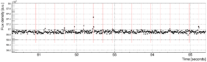
Caption : Example de-dispersed time series from the data recorded on 2023-02-01/02 with bright pulses from the pulsar B0950+08. Red dashed lines separated by the pulsar period (approximately 0.253 seconds) mark the expected pulse arrival times. A very bright pulse at the time 92.44 seconds since the start of the observation is clearly visible and several fainter pulses can be seen as black dots on top of red dashes lines. The X-axis is time since the start of the observation and Y-axis is flux density in arbitrary units (hence [a.u.]).